Splines Model
Introduction
Splines can be used to model relationships between data points where a strict mathematical model is unknown or impossible. Splines of order N over K knots are defined as pieces of Nth order polynomials between the knots. The polynomial pieces and its N-1 derivatives are all continuous on the knots locations. We call this property N-smooth. The spline model is defined over a finite domain. The knots can be located anywhere in the domain provided that there is one knot at the minimum of the domain and one knot at the maximum.
The behaviour of splines of different orders is explained in the table.
| order | Behaviour between Knots | Continuity at Knots |
|---|---|---|
| 0 | piecewise constant | not continuous at all |
| 1 | piecewise linear | lines are continuous (connected) |
| 2 | parabolic pieces | 1st derivatives are also continuous |
| 3 | cubic pieces | 2nd derivatives are also continuous |
| n>3 | n-th order polynomials | (n-1)-th derivatives are also continuous |
The most often used splines are cubic splines on a regular grid of knots.
From here on we work with cubic splines on a random grid unless otherwise indicated. It is quite easy to extend the ideas to lower or higher orders.
Simple Spline.
My first implementation of splines were based on this continuity only.
Assume we have a set of knots as in
|------------|------|---------|-------------------|---
k0           k1     k2        k3                  k4   etc..
The set of knots defines the domain where the spline model is valid.
We define a 3rd order polynomial to the first knot segment $(k_0,k_1)$
 |
(1) |
|---|
Where x0 is the distance to k0 : x0 = x - k0.
For the second segment (k1,k2) we extend the function of the previous segment and add
 |
(2) |
|---|
where x1 is the distance to k1 : x1 = x - k1.
Note that the function f1 is continuously differentiable to the 3rd derivative. For x < k1 it is all 0; for x > k1 it is a 3rd order polynomial and at x = k1 the derivatives from the up-side are all 0, equal to those from the low-side.
For the next segments we repeat this procedure.
So in the end we have a spline function f(x) as
 |
(3) |
|---|
Obviously this (piecewise) function is continuously differentiable to the 3rd derivative as it is a sum of continuously differentiable functions. So it is a valid cubic spline model.
symmetric. We could also have started at the end of the domain and worked our way to the beginning. We would obtain a different spline representation, not better or worse than the first. Secondly the parameters are not localized. Each parameter influences the result over the rest of the domain. Preferably one parameters affects only one part of the model without influencing the others. In this algorithm a parameter affects all later parameters.
Even with these defects it is a usefull and fast algorithm. The algorithm is implemented in SplinesModel.
In figure 1 the model is displayed with all its components.

| Figure 1 shows the the splines model and all its components. The knots are located at (0,2,4,6,8,10). |
Figure 1 is made with the following piece of python code.
from BayesicFitting import SplinesModel
import matplotlib.pyplot as plt

x = numpy.linspace( 0, 10, 101, dtype=float )
kn = numpy.linspace( 0, 10, 6, dtype=float )
sm = SplinesModel( knots=kn )

par = [1.989, 0.066, 0.010, 0.016, -0.046, -0.028, 0.210, -0.286]
sm.parameters = par

part = sm.partial( x, par )
yf = numpy.zeros( 101, dtype=float )
for k in range( sm.npars ) :
    yf += part[:,k] * par[k]
    plt.plot( x, yf )

plt.plot( x, sm.result( x, par ), 'k-' )
plt.title( "Splines model and its constituents" )
plt.show()
Basis Splines.
To address the defaults of simple splines, basis splines were invented. They consist of a set of base functions that, linearly combined, form the required functional relation.
Carl de Boor (in "A Practical Guide to Splines.", (1978) Springer-Verlag. ISBN 978-3-540-90356-7.) designed a recursive algorithm where each recursion produces a set of base splines of a higher order.
John Foster and Juha Jeronen implemented de Boor's algorithm in Python in the bspline package. We encapsulated the bspline package into our BSplinesModel.
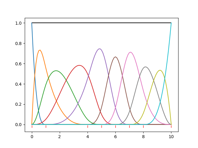
In figure 2 a set of basis splines of order 3 is displayed, using parameters all equal to 1.0. The knots are at (0,1,4,5,6,7,8,10). 8 knots resulting in 10 basis functions and as many parameters. The sum of the components is the black line constant at 1.0.
 |
|---|
|
Figure 2 shows the de Boor splines model and all its components. The position of the knots is indicated with red bars low in the plot. |
Unfortunately the recursive implementation in BsplinesModel is about 20 times slower than the the splines in SplinesModel.
Constructing a Basis.
We would like to see whether the continuity approach can be applied to these basis functions. we will explain the construction of cubic (3-order) splines on a set of arbitrarily spaced knots, where the number of knots is larger than the order.
First Blob
Looking at figure 2, we observe that the first (blue) blob runs only in the first knot segment. It is unbound (0-smooth) at the left side and 3-smooth with 0 at the right side.
We have a 3rd order polynomial between the first 2 knots.
 |
(4) |
|---|
      f1
|------------|----
x0          x1
The property 3-smooth implies that the function and it first and second derivative are 0 at x1, while the function is unbound, arbitrary at x0. We normalize the blob in x0 at 1.
 |
(5) |
|---|
Now we have 4 equations with 4 unknown coefficients (a,b,c,d) which we can solve.
Second Blob.
The second blob is defined over two knot segments. In each segment a 3rd order polynomial function is defined: f1 and f2. Note that this function, f1, are different from the f1 of the first blob.
     f1           f2
|--------------|--------|---
x0            x1      x2
 |
(6) |
|---|
The function, f1 is 1-smooth at x0, i.e. touching zero; f1 and f2 are 3-smooth at x1, and f2 is 3-smooth with 0 at x2. Again we need a normalization at x1 for both f1 and f2.
 |
(7) |
|---|
We have 8 equations and 8 coefficients (4 per function) so it can be solved directly.
Next Blobs.
A pattern is developing. The next blob is 2-smooth at x0, and 3-smooth at all other knots, resulting in 12 polynomial coefficients. The ones after that are 3-smooth everywhere over 4 knot segments, resulting in 16 coefficients. Until the end where the pattern is the reverse of the one at the start.
Renormalization
The normalization that we applied on the individual knots is not exactly what we want, although it is perfectly valid and we could use it as is. We would rather have the blobs such that a constant line at 1.0 would be the result when all parameters are set to 1.0.
So we calculate the results at the top position of the blobs (more or less; it does not matter that much as is should be 1 everywhere) and set all these results to 1.0. This is a matrix equation of size nrknots, and can be solved directly.
Small number of knots
In case we have a cubic spline on a set of 2 knots, x0 and x1, we have 4 blobs. The smoothnes at the knots is given in the table below.
| blob | x0 | x1 |
|---|---|---|
| 1 | 0-smooth | 3-smooth |
| 2 | 1-smooth | 2-smooth |
| 3 | 2-smooth | 1-smooth |
| 4 | 3-smooth | 0-smooth |
In case we have a cubic spline on a set of 3 knots, x0, x1 and x2, the smoothnes of the blobs at the knots is given in the table below.
| blob | x0 | x1 | x2 |
|---|---|---|---|
| 1 | 0-smooth | 3-smooth | n/a |
| 2 | 1-smooth | 3-smooth | 3-smooth |
| 3 | 2-smooth | 3-smooth | 2-smooth |
| 4 | 3-smooth | 3-smooth | 1-smooth |
| 5 | n/a | 3-smooth | 0-smooth |
It is easy to generalize the behaviour for splines of other orders.
Algorithm
The construction above is implemented in BasicSplinesModel. Up on initialization of the class all polynomial coefficients are calculated and normalized. This takes some time, but after that the calculation of the spline results, S, is fast.
In the model each blob fk has assigned a parameter pk.
 |
(8) |
|---|
We can expand the fk into its blob coefficients.
 |
(9) |
|---|
And then multiply and sum the parameters and coefficients to speed up the calculations.
 |
(10) |
|---|
The coefficients and the parameters can be multiplied together, forming one piecewise 3-order polynomial function of the x's.
This algorithm proved to be 10 times faster than the recursive one. Still slower by a factor 2 than the first one.
when one parameter changed only localized effects are seen. Even when the position of a knot shifts, adjacent knots are only slightly affected. This opens the option of a SplinesDynamicModel.