Navigation

Global	Documentation
Home	Manual
Readme	Glossary
Notes	Design
Examples	Classes
	Trouble
	Style

Contents

Content
1. Introduction
2. Model Classes
3. Fitter Classes
4. Nested Sampling
5. References

 

Architectural Design Document.

1. Introduction

The BayesicFitting package offers a general way to fit models to data in a Bayesian way. It consists of 3 families of classes: the Model classes, the Fitter classes and the NestedSampling classes.

This is not the place to explain either the mathematics behind Bayesian modelling of data or the algorithms used. For the mathematics look at the books of Sivia, Bishop, von der Linden and Jaynes and for some fitter algorithms Press.

2. Model Classes.

The Model classes define the model functions which are to be fitted. A model class has methods to return its function value and partial derivates given one input value and a set of parameters. It is also the place where the parameters and standard deviations are stored once they are fitted. Limits on the allowed parameter range belong to the model domain too. Just like fixed parameters.

A partial and schematic view on the model classes and their relationships can be found in figure 1.

For all images it holds that the boxes are classes. In the upper panel the name, in the mid panel some of the attributes of the class and in the lower panel some methods. Not all attributes and methods are displayed. An open arrow indicates inheritance: Model inherits from FixedModel which inherits from BaseModel. A black arrow indicates a relationship between the classes, which is written next to it.

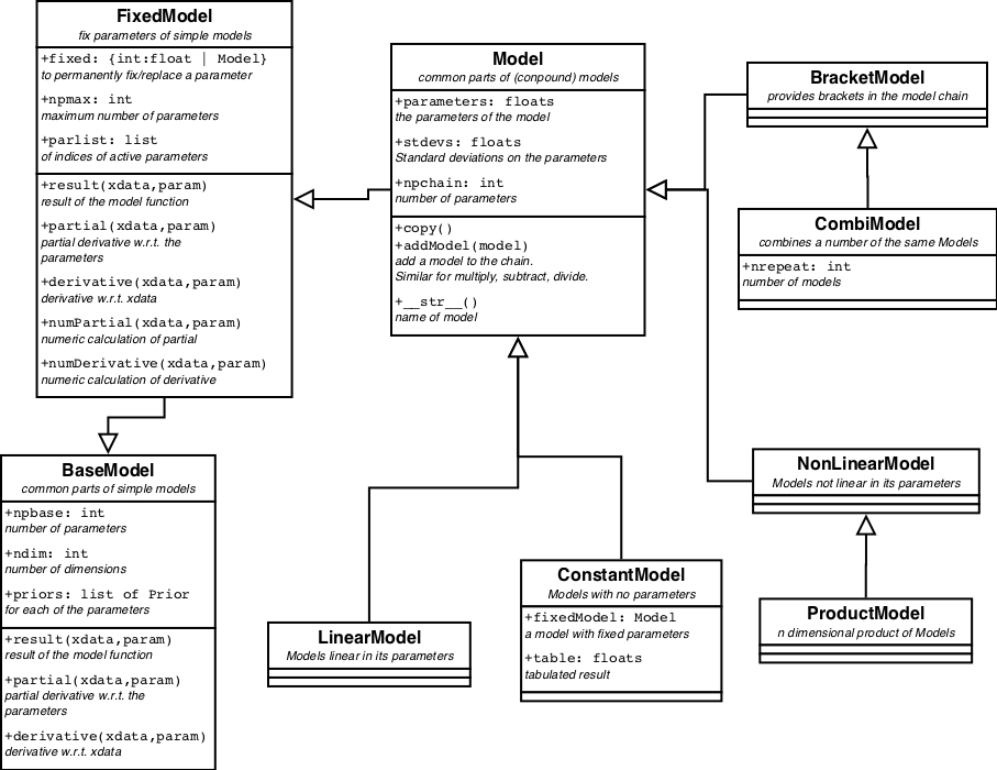
Figure 1. Class hierarchy diagram for models. Blue boxes refer to further hierachy diagrams.

BaseModel.

BaseModel defines a simple or basic model and all its methods. A basic model has methods to return the functional result, y = f( x:p ), where p represents the parameters; it is an array (or list) of K floats. x is the independent variable. It can have any length, even being a single number. If the model is more-dimensional, x needs to have 2 dimensions, an array of points in a more-dimensional space. The shape of x is N or (N,D), where N is the number of points and D (>=2) is the dimensionality. y is the result of the function. It has a length of N, irrespective of the dimensionality of the model. If the BaseModel can handle it, the x variable can even be a list of different types. No pre-defined model in this package is like that, but a user might see some usage for it.

BaseModel also defines the partial derivatives of f to p, ∂f(x:p) / ∂p and derivatives of f to x. The shapes are resp. (N,K) and N or (N,D). When no (partial) derivatives can be calculated, this class automatically provides numerical (partial) derivatives. The derivative, ∂f / ∂x, is only used when models are connected via a pipe operation. See Model. However, the partials, ∂f / ∂p, are intensively used by the fitters to feel its ways towards the minimum.

Each BaseModel provides its own name and names for its parameters.

BaseModels reach out to concrete implementations of simple models, see Figures 2 and 3, via methods called baseResult, basePartial, baseDerivative and baseName, to get the there implemented result, partial etc.

FixedModel.

In each BaseModel one or more parameters can be replaced either by a constant or by another Model. This is handled in FixedModel. For each fixed parameter, the model loses one item in the parameter list. When the parameter is replaced by a Model, the parameters of the Model are appended to the BaseModels parameter list; in the same order as they are provided.

FixedModels stay fixed for as long as the object exists. Consequently they can only be constructed when the BaseModel itself is constructed. Models can only be fixed up on construction.

Results and partial derivatives for FixedModels are calculated from the constituent Models. The derivative to the independent variable cannot be calculated in general. They are replaced by numeric derivatives.

A FixedModel is still a simple model, even though quite elaborate functionality can be constructed this way.

Model.

In the center of the tree sits Model, the last common anchestor of the model classes. It is the class that fitters and nested sampling work up on. A Model needs to define all methods that the fitters might need, in particular the methods result( xdata, parameters ) and partial( xdata, parameters ), where xdata and parameters are the x and p in f( x:p ) as defined above.

It also contains methods for keeping some of the parameters fixed, temporarily during the fitting, for checking for positivity of some parameters and/or non-zeroness and for applying limits on the parameters.

Two or more models can be concatinated to form a new compound model with model1 + model2. The result equals the sum of the individual results. The parameters are listed with the ones from model1 first, followed by those of model2, etc. Other arithmetic operators (-*/|) can be used too, with obvious results.

The methods of a compound model are called recursively over the chain.

For every (simple) model in a chain. relevant information is kept within the Model itself: lists of parameters, standard deviations (when available) and Priors. The latter ones are only seriously used when the Model is used in NestedSampler.

After the Model things starts to diversify into different directions, LinearModels and NonLinearModels, AstropyModels and UserModels, the BracketModel and the ConstantModel.

BracketModel.

BracketModel provides brackets () in the model chain. It enables to distinguish between m1 * m2 + m3 and m1 * (m2 + m3). In the model chain the models are handled strictly left to right, so m1 + m2 * m3 is implemented as (m1 + m2 ) * m3. The BracketModel can change the order of calculation where that is needed.

CombiModel.

A CombiModel combines a fixed number of Models into one, while maintaining certain relations between similar parameters. E.g. to fit a triplet of lines in a spectrum, combine 3 line models (GaussModel) into a CombiModel with all the same linewidths and the known distances of the lines in the triplet. This way there are only 5 parameters (3 amplitudes, 1 position and 1 width) to be fitted. See Example (TBD)

ConstantModel.

ConstantModel is the first concrete child of Model. It returns a constant form, no matter what the input. The constant form could be 0 everywhere, but also another Model with known parameters, or even a table.

AstropyModel.

AstropyModel is a wrapper around a FittableModel from the astropy library, astropy.modeling.FittableModel. When wrapped, the astropy models can be used as a simple model in all tools provided by BayesicFitting.

UserModel.

UserModel is a wrapper around a user-supplied python method returning the result for a model. Optionally also partial and derivative methods can be supplied. A UserModel can be used as a simple model in all tools BayesicFitting provides.

Linear Models.

LinearModels are linear in its parameters, meaning that the result of a concrete linear model is the inner product of the partial derivatives with the parameters. This operation is defined in this class. Consequently concrete linear models only need to define the partials as basePartial.

All pre-defined linear models are displayed in figure 2

Figure 2. Class hierarchy diagram for linear models.

LinearModels have quite some benefits. Using a Gaussian error distribution (aka least squares) the optimal parameters can be found directly by `inverting' the Hessian matrix. Computationally there are several methods to achieve it, which are all relatively simple. They are implemented in the linear fitter classes. Another benefit is that the posterior for the parameters is also a multidimensional Gaussian, which is completely characterized by its covariance matrix and can be easily integrated to obtain the evidence.

It is not wrong to use a non-linear fitter on a linear model. Sometimes it can even be necessary e.g. when the number of parameters gets large.

Non Linear Models.

All Models that are not linear are NonLinearModels. They at least need to define the result as baseResult. When basePartial or baseDerivative is not implemented, numeric approximations are used.

All pre-defined non-linear models are displayed in figure 3

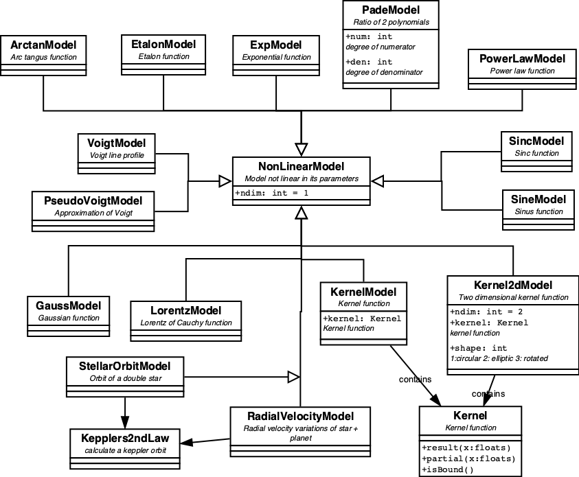
Figure 3. Class hierarchy diagram for non-linear models.

NonLinearModels need non-linear (NL) fitters to optimize their parameters. As NL fitters are iterative, more complicated, slower and not guaranteed to find the best solution, NonLinearModels are harder to handle.

Dynamic and Modifiable.

Dynamic and/or Modifiable models are specialisations of Models with some fixed attribute. E.g PolynomialModel with fixed degree or SplinesModel with fixed knot list. Dynamic implements methods to let the model grow or shrink.
Modifiable implement a method to vary the internal structure of the model, e.g. vary the knot location in a BasicSplinesModel*. Dynamic cq. modifiable models inherit from Model but also from Dynamic and maybe from Modifiable. They have more than one parent class.

These models can not be used with ordinary Fitters. Using NestedSampler they automatically converge on the model with the optimal number of components.

All pre-defined Dynamic and Modifiable models are displayed in figure 4.

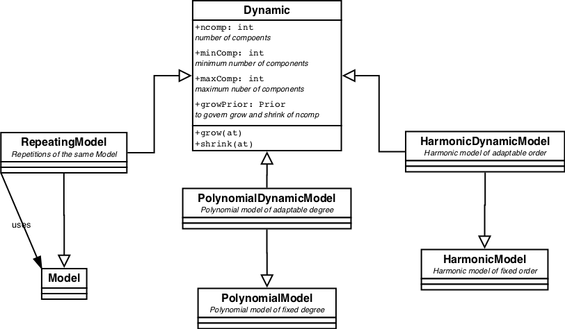
Figure 4. Class hierarchy diagram for dynamic and modifiable models.

KernelModels.

A special case of NonLinearModels are the KernelModels and their more-dimensional variants, Kernel2dModel. A KernelModel encapsulates a Kernel function, which is defined as an even function with a definite integral over (-inf,+inf).

All pre-defined kernels are displayed in figure 5.

Figure 5. Class hierarchy diagram for kernels.

Of the more-dimensional variants, only the 2-dim is defined, where the 2d kernel is either round or elliptic along the axes, or rotated elliptic. For more-dimensional kernels some kind of rotational matrix needs to be defined. It more or less waits for a real case where it is needed.

Note that GaussModel and LorentzModel could both be implemented as a KernelModel, while SincModel actually is a wrapper around a KernelModel.

Construction of new Models.

If a newly required model can not be constructed via the fixing of parameters or by concatenating models, it is advised to take a similar (linear or non-linear) model as an example and change the revelant methods. As a bare minimum the method baseResult need to be filled. The method basePartial either needs to be filled or the method should be removed. In the latter case numeric derivatives are used. A simple alternative is the UserModel.

The method testPartial in Model can be used to check the consistency between the methods baseResult and basePartial.

When a new model is constructed either from existing ones or new, it is the users responsibility to make sure the the parameters are not degenerate, i.e. measuring essentially the same thing.

3. The Fitter Classes.

BaseFitter.

The root of the fitter classes is BaseFitter, a large class containing the common methods for parameter fitting. Mostly these are methods using the covariance matrix, like calculating the standard deviations or the confidence regions of the fit. And most importantly the calculation of the evidence. This is done by a Gaussian approximation of the posterior, also known as Laplace's method. For the prior a UniformPrior is asumed, for which limits are necessary to make it a proper probability. The limits need to be provided by the user.

In case of parameter estimation of a LinearModel, Laplace's method is exact, provided that the limits on the parameters are wide enough. In all other cases it is an approximation, better or worse depending on the problem at hand. Nontheless it can be used succesfully in model comparison when some reasonable provisions are taken into account, like comparing not too different models, feeding the same data (and weights) to all models etc.

The Fitter inheritance tree is displayed in figure 6.

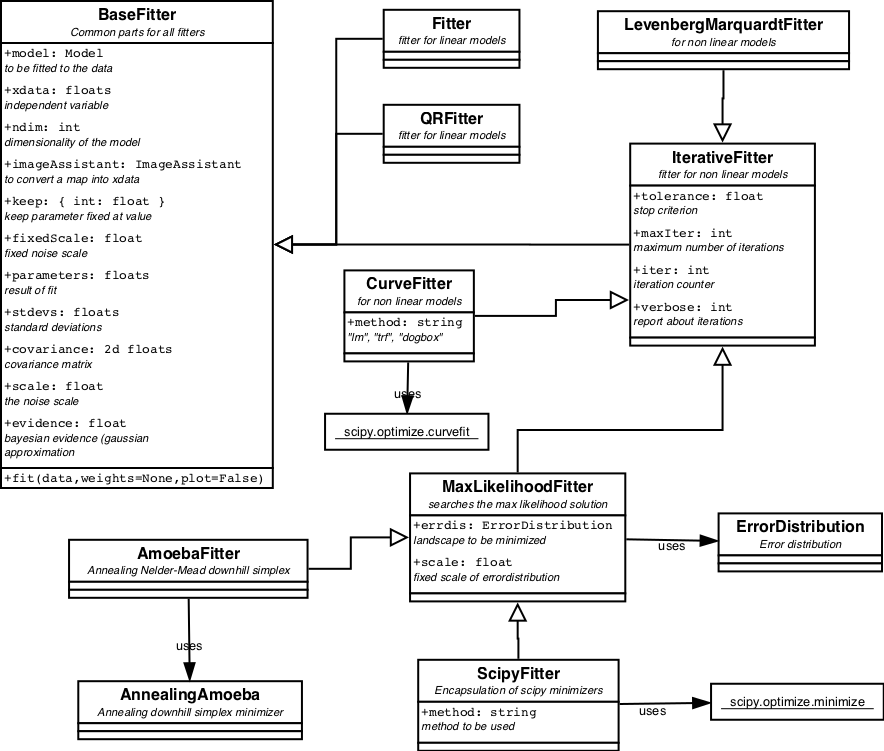
Figure 6. Class diagram for the fitters. Dark red boxes refer to methods of SciPy, outside the scope of BayesicFitting.

Linear Fitters.

The package contains 2 linear fitter classes: Fitter and QRFitter. The former applies LU-decomposition of the Hessian matrix and is best for solving single problems. The latter applies a QR-decomposition of the Hessian. When the same problem needs to be solved for several different datasets QR-decomposition is more efficient.

A third method, Singular Value Decomposition (SVD), is somewhat more robust when the Hessian is nearly singular. SVD decomposes the design matrix into a singular value decomposition. Those singular values which do not exceed a threshold are set to zero. As a consequence the degenerate parameters get values which are minimalised in a absolute sense.

The SVD-Fitter is TBW.

NonLinear Fitters.

The other descendants of the BaseFitter are all iterative fitters to be used with non-linear models. IterativeFitter implements a number of methods common to all non-linear fitters.

Non-linear fitters are iterative, take more time and have no guarantee that it will find the global optimal. Most NL fitters fall in the first local minimum and can not escape from there. These fitters can only be used effectively on problems where the global minimum is close by; either because the problem has only one minimum (it is monomodal), or the initial parameters are close to the final global minimum. When uncertain about it, one could start the fitter at widely different initial positions and see whether it ends up at the same location.

LevenbergMarquardtFitter.

The LevenbergMarquardtFitter is an implementation of Levenberg-Marquardt algorithm from Numerical Recipes par. 15.5. It actively uses the partial derivatives. The LevenbergMarquardtFitter will go downhill from its starting point, ending wherever it will find a minimum. Whether the minumum is local or global is unclear.

CurveFitter.

CurveFitter ecapsulates the method scipy.optimize.curvefit. See curvefit for details.

MaxLikelihoodFitter.

Up to now all fitters try to find the minimum in the χ²-landscape. They are strictly "least squares". MaxLikelihoodFitters can also maximize the log likelihood of a selected ErrorDistribution.

AmoebaFitter.

The AmoebaFitter performs the simplex method described in AnnealingAmoeba to find the minimum in χ² or the maximum in the likelihood.

AnnealingAmoeba.

AnnealingAmoeba implements the simplex method designed by Nelder and Mead to find the minimum value in a functional landscape. In its simple invocation with temperature = 0, it proceeds downhill only in the functional landscape. Steps where the value increases are refused so it falls and stays in the first minimum it encounters. In that respect it has the same limitations as the LevenbergMarquardtFitter.

The implementation here adds Metropolis annealing to it: Depending on the temperature it sometimes takes steps in the uphill direction, while downhill steps are always taken. Gradually the temperature diminishes. This way it might escape from local minima and find the global minimum. No guarantee however. In doubt start it at different initial values etc.

AnnealingAmoeba evolved from earlier implementations of the Nelder-Mead algorithm in [Press][5] par 10.4 and 10.9.

ScipyFitter.

The method scipy.optimize.minimize implements about 10 minimization algorithms. ScipyFitter encapsulates the minimize method and call the algorithms by their name. However there are also 10 named fitters all residing within ScipyFitter.

They are presented here as is. We dont have much experience with most of them, except with the ConjugateGradientFitter.

ConjugateGradientFitter.

The ConjugateGradientFitter is especially usefull when there are many (>20) parameters to be fitted, as it does not require matrix manipulations. For models with very many parameters (>10000) where construction of the Hessian matrix starts to run out of memory, it is possible to implement the gradient method directly in the model.

The others are NelderMeadFitter, PowellFitter, BfgsFitter, NewtonCGFitter, LbfgsFitter, TncFitter, CobylaFitter, SlsqpFitter, DoglegFitter and TrustNcgFitter.

For details on the individual ScipyFitters see minimize

RobustShell.

In real life data often outliers are present, little understood large excursions from the general trend. It also can occur that some parts of the data need to be excluded from the fit, e.g. because at those places there is flux and the fit should be only to the background. In those cases RobustShell is usefull. RobustShell is a shell around a Fitter. In an iterative way it de-weights the outliers. Kernel functions can be used as de-weighting schemes.

Robust fitting is even more error prone than normal fitting. Always carefully check the results.

4. NestedSampler.

Nested Sampling is an algorithm invented by David MacKay and John Skilling, to integrate the posterior to obtain the evidence. At the same time samples from the posterior are collected into a SampleList. NestedSampler follows the core algorithm as presented in Sivia closely, but is expanded with pluggable Problems, Models, Priors, ErrorDistributions and Engines. It offers solutions to a wide variety of inverse problems.

Initially an ensemble of points representing the parameters, is randomly distributed over their priors. These points are called walkers and typically there are 100 of them. They are collected in a WalkerList.

In an iterative loop, the walker with the lowest likelihood is removed from the ensemble of walkers. It is weighted and stored as a Sample in the SampleList. One of the remaining walkers is copied and randomly moved around by Engines, provided that its likelihood stays higher than that of the stored Sample. This way the walkers slowly climb to the maximum value of the likelihood. The stored Samples provide enough pointers into the Likelihood function to make a good estimate of the integral (evidence).

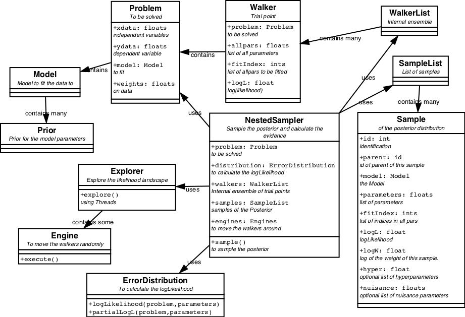
Figure 7 Class diagram for NestedSampler.

The classes associated with NestedSampler are displayed in figure 7.

Descendants.

NestedSampler has two descendants. The first is PhantomSampler. Phantoms are the points in parameter space that are visited by the engines in their quest to randomize the copied walker.
PhantomSampler uses all phantoms in the calculation of the evidence. By default it has an ensemble of 20 walkers, making it faster. The coarse integration steps are filled in by the phantoms.

The second descendant arises from the realization that the nested sampling algorithm is also a maximum finder. When some kind of cost function can be defined for each parameter configuration, the maximum can be found. That leads to NestedSolver. Upto now there is only the travelling salesman in SalesmanProblem using a DistanceCostFunction. School schedules, sports competitions etc. also belong to this category. They would need specialized CostFunctions and also specialized OrderEngines.

The classes inheriting from NestedSampler are in figure 8.

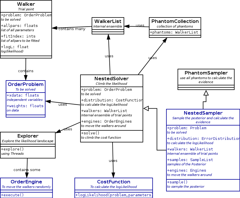
Figure 8. Classes inheriting from NestedSampler.

Problems.

NestedSampler acts upon a Problem. A Problem is a object that encodes a solvable problem. This is meant in a very broad sense. The solution of the problem is contained in the parameters. Together with (special) ErrorDistribution, Engines and Priors, NestedSampler can optimize the parameters. What the Problem, parameters, etc. exactly are, is completely dependent on the problem to be solved.

In versions before 2.0 of this package, only problems with parameterized models, and one-dimensional outputs were handled. For these kind of problems ClassicProblem is introduced. Mostly it operates behind the scenes and is invisible for the users.

IN version 2 the concept of a Problem was introduced to handle more complicated cases. We have the MultipleOutputProblem for problems with more dimensional output, like a steller orbit on the sky, selection in categories, football matches etc. A further specialization is the FlippedDataProblem (not yet in this version) where there might be ambiguity in the stellar orbit data.

Classically it is assumed the xdata are known with a much higher precision than the ydata. For cases where this is not met, we have the ErrorsInXandYProblem. Now the true positions of the xdata have to estimated too. ErrorsInXandYProblem introduces extra problem parameters for all xdata positions. All these extra parameters need a Prior. They are all optimized along with the model parameters. And subsequently ignored. They are called nuisance parameters.

The EvidenceProblem is not about optimizing parameters, but about optimizing Models. We need Modifiable models and optimize the structure of the model by finding the one with the best evidence. The error distribution for this problem is called ModelDistribution.

And finally we have the OrderProblems where the parameters to be optimize might be something much more convoluted than a simple list of numbers. OrderProblems need their own Engines. They need an ErrorDistribution in the form of a CostFunction. OrderProblems are not strictly Bayesian, unless the CostFunction is a true distribution.

The class diagram for Problems can be found in figure 9.

Figure 9. Class hierarchy diagram for problems.

A Problem has Priors for all its parameters. Itknows how to calculate its result, partial and derivative given the parameters. It also knows which Engines and which ErrorDistribution is the best choice.

Priors.

The Priors contain information about the parameters which is known before the data is taken into account. It is the range that the parameters can move, without being frowned up on.

The predefined Priors are displayed in figure 10.

Figure 10. Class hierachy diagram for priors.

All Priors define two methods unit2domain which transforms (random) value in [0,1] into a (random) value from the prior distribution, and its inverse domain2unit.

All Priors can have limits, cutting off part of the domain. Symmetric ones can also be defined as circular, folding the high limit on to the low limit, or using a center and a period.

ErrorDistributions.

The main task of the ErrorDistribution is to calculate the likelihood, or better the log thereof. The partial derivative of the log( likelihood ) with respect to the parameters is also defined. It is used in the GalileanEngine.

The predefined ErrorDistributions are displayed in figure 11.

Figure 11. Class hierachy diagram for error distributions.

Some ErrorDistributions have parameters of themselves, so called HyperParameters. One special case is the NoiseScale.

NoiseScale.

The NoiseScale contains information about the amount of noise in the data. This can be in the form of a fixed number, claimimg that the amount of noise is known beforehand. Or it can be in the form of a prior. As the amount of noise is a positive definite number, the non-informative prior for it is the JeffreysPrior. The JeffreysPrior is, like the UniformPrior, an improper prior, which means that its integral is unbound. Low and high limits (both > 0) need to be provided when calculating the evidence.

Engines.

The way the walkers are moved around in the available parameter space is determined by the Engines. Several Engines are availble: ChordEngine, GalileanEngine, GibbsEngine, and StepEngine. For Dynamic models, the BirthEngine and the DeathEngine are needed. And for Modifiable models, the StructureEngine is needed.

The available Engines are displayed in figure 12.

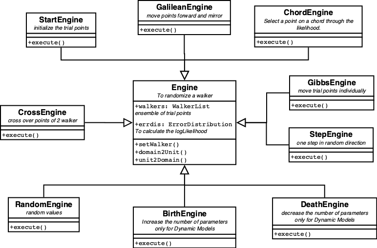
Figure 12. Class hierachy diagram for engines.

The StartEngine generates the initial random ensemble. It is called before the iterations start.

Two engines need special mentioning. The GalileanEngine moves the point in a random direction for several steps. When the walker is moving outside the area defined by the lowest likelihood, the direction is mirrored on the likelihood boundary.
The ChordEngine selects a random line through the present point until it reaches outside the allowed space. Then it moves to a random point on the line, while staying inside the allowed space. And repeats until done.

Ordering Engines

For ordering problems a different set of engines is required. The ones listed here are most probable only usefull for the SalesmanProblem. For other, e.g. scheduling problems, specific engines must be written.

The classes for traveling salesman engines are listed in figure 13.

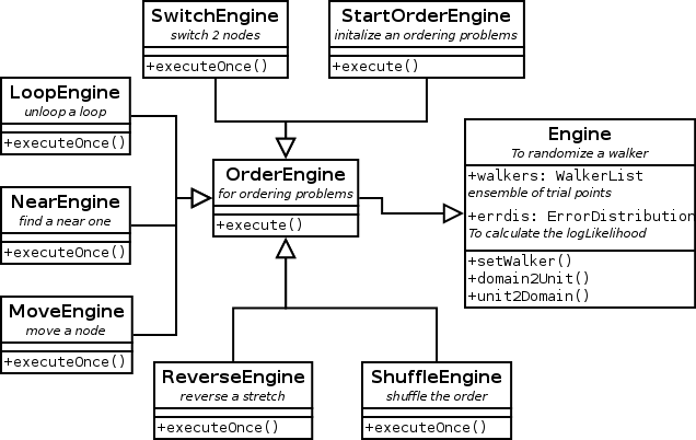
Figure 13. Class hierachy diagram for order engines.